1. Getting Started With Robot Inverse Kinematics (IK)#
Welcome to the first guide in the series of getting started with Dr.QP robot Inverse Kinematics (IK). In this guide, we will cover the basics of IK and how to use it to control a robot.
What is Inverse Kinematics?#
Inverse Kinematics (IK) is a technique used in robotics to determine the joint angles required to achieve a desired end-effector position. It is the process of solving the inverse problem of forward kinematics, which calculates the end-effector position given the joint angles.
Why is Inverse Kinematics Important?#
Inverse Kinematics is important because it allows robots to perform complex movements and tasks. By calculating the joint angles required to reach a specific position, robots can navigate their environment and interact with objects more effectively. In case of Dr.QP robot, it allows to generate gaits and move around in a desired way as well as moving its body in space.
How to Use Inverse Kinematics#
To use Inverse Kinematics, you need to have a model of your robot’s kinematics. This model includes the lengths of the robot’s links and the joints. Once you have this model, you can use it to calculate the joint angles required to achieve a desired end-effector position.
The robot model#
For this tutorial we will use the simplest part of Dr.QP robot - a single leg.
It has a 3 degrees of freedom and consists of 3 links:
coxa (hip)
femur (thigh)
tibia (shin)
and 3 joints:
alpha (coxa joint, hip joint)
beta (femur joint, thigh joint)
gamma (tibia joint, shin joint)
Links have only single property - length. They are connected to each other with joints. Joints have only single property - angle.
The diagrams below will make it much more clear, I promise.
The values below are the default parameters for the simulated leg used in this tutorial.
coxa_length = 5
femur_length = 8
tibia_length = 10

alpha = 0  # controls coxa angle, 0 is straight
beta = 0  # controls femur angle, 0 is straight
gamma = 0  # controls tibia angle, 0 is straight
Forward kinematics#
Before we dive into the details of how inverse kinematics works, let’s first get familiar with forward kinematics. The forward kinematics of the robotic leg is the process of calculating the position of the foot based on the angles of the joints.
Coxa, femur and tibia are represented with vector that is rotated at its base. Each next link starts at the ened of the previous link.
from drqp_kinematics.geometry import Line, Point


# unused
def forward_kinematics_rads(
    coxa_length,
    femur_length,
    tibia_length,
    alpha_rad,
    beta_rad,
    gamma_rad,
    start_height=2,
    body_length=3,
):
    start = Point(0, start_height)
    body = start + Point(body_length, 0, f'{alpha_rad=}rads')
    coxa = body + Point(coxa_length, 0, f'{beta_rad=}rads').rotate(alpha_rad)
    femur = coxa + Point(femur_length, 0, f'{gamma_rad=}rads').rotate(beta_rad)
    tibia = femur + Point(tibia_length, 0, 'Foot').rotate(gamma_rad)

    return (
        Line(start, body, 'Body'),
        Line(body, coxa, 'Coxa'),
        Line(coxa, femur, 'Femur'),
        Line(femur, tibia, 'Tibia'),
    )
Radians is a natural way to represent angles in most of the math related to robotics, however I find it easier to think in degrees, therefore I will be using degrees in this notebook.
import numpy as np


def forward_kinematics(
    coxa_length,
    femur_length,
    tibia_length,
    alpha,
    beta,
    gamma,
    start_height=2,
    body_length=5,
    verbose=False,
):
    alpha_rad = np.radians(alpha)
    beta_rad = np.radians(beta) + alpha_rad
    gamma_rad = np.radians(gamma) + beta_rad

    start = Point(0, start_height)
    body = start + Point(body_length, 0, rf'$\alpha$={alpha}°')
    coxa = body + Point(coxa_length, 0, rf'$\beta$={beta}°').rotate(alpha_rad)
    femur = coxa + Point(femur_length, 0, rf'$\gamma$={gamma}°').rotate(beta_rad)
    tibia = femur + Point(tibia_length, 0, 'Foot').rotate(gamma_rad)

    result = (
        Line(start, body, 'Body'),
        Line(body, coxa, 'Coxa'),
        Line(coxa, femur, 'Femur'),
        Line(femur, tibia, 'Tibia'),
    )

    if verbose:
        print(f'{start=}')
        print(f'{body=}')
        print(f'{coxa=}')
        print(f'{femur=}')
        print(f'{tibia=}')

        for line in result:
            print(line)

    return result
First, lets see how our leg looks in the neutral position. It is a straight line going from start point at (0, 0) and ending with the Foot
from plotting import plot_leg_with_points

model = forward_kinematics(coxa_length, femur_length, tibia_length, alpha, beta, gamma)

_ = plot_leg_with_points(model, 'Neutral position (straight leg)')
display_and_close(plt.gcf())

Now lets try changing some angles to see how it behaves. Feel free to experiment with different values.
model = forward_kinematics(coxa_length, femur_length, tibia_length, 50, -60, -10)

_ = plot_leg_with_points(
    model, 'Lifted up (coxa) and bent down (femur, tibia)', link_labels='legend'
)
display_and_close(plt.gcf())

# Lifted up (coxa) and bent down (femur), with foot on the ground (guessed angle)
model = forward_kinematics(coxa_length, femur_length, tibia_length, 45, -55, -14)

_ = plot_leg_with_points(model, 'Foot on the ground', link_labels='legend')
display_and_close(plt.gcf())

Exercise 1. Forward kinematics. Find angles at which the leg is on the ground#
Its time to have a little fun with our robot.
Using the sliders on the interactive diagram below try to find angles at which the foot is on the ground.
from plotting import animate_plot, plot_leg_update_lines

start_height = 3
alpha = 0
beta = 35
gamma = -110
model = forward_kinematics(
    coxa_length,
    femur_length,
    tibia_length,
    alpha,
    beta,
    gamma,
    start_height=start_height,
)

frames_to_animate = 50

fig, _, plot_data = plot_leg_with_points(
    model,
    'Find angles to place foot on the X axis',
    link_labels='legend',  # if is_interactive else 'inline',
    joint_labels='points',  # if is_interactive else 'annotated',
)


def animate(frame=0, alpha=alpha, beta=beta, gamma=gamma):
    if frame > 0:
        beta = np.interp(frame, [0, frames_to_animate / 2], [35, 55])
        gamma = np.interp(frame, [frames_to_animate / 2, frames_to_animate], [-110, -140])

    model = forward_kinematics(
        coxa_length,
        femur_length,
        tibia_length,
        alpha,
        beta,
        gamma,
        start_height=start_height,
    )
    plot_leg_update_lines(model, plot_data)
    fig.canvas.draw_idle()


_ = animate_plot(
    fig,
    animate,
    _interactive=True,
    _frames=50,
    alpha=(-180, 180, 0.1),
    beta=(-180, 180, 0.1),
    gamma=(-180, 180, 0.1),
)

# If plot is not responding to changes in sliders, most likely figure was closed. Rerun this cell to reactivate it.
---------------------------------------------------------------------------
RuntimeError                              Traceback (most recent call last)
File ~/checkouts/readthedocs.org/user_builds/drqp/checkouts/latest/.venv/lib/python3.12/site-packages/IPython/core/formatters.py:406, in BaseFormatter.__call__(self, obj)
    404     method = get_real_method(obj, self.print_method)
    405     if method is not None:
--> 406         return method()
    407     return None
    408 else:

File ~/checkouts/readthedocs.org/user_builds/drqp/checkouts/latest/.venv/lib/python3.12/site-packages/matplotlib/animation.py:1385, in Animation._repr_html_(self)
   1383 fmt = mpl.rcParams['animation.html']
   1384 if fmt == 'html5':
-> 1385     return self.to_html5_video()
   1386 elif fmt == 'jshtml':
   1387     return self.to_jshtml()

File ~/checkouts/readthedocs.org/user_builds/drqp/checkouts/latest/.venv/lib/python3.12/site-packages/matplotlib/animation.py:1302, in Animation.to_html5_video(self, embed_limit)
   1299 path = Path(tmpdir, "temp.m4v")
   1300 # We create a writer manually so that we can get the
   1301 # appropriate size for the tag
-> 1302 Writer = writers[mpl.rcParams['animation.writer']]
   1303 writer = Writer(codec='h264',
   1304                 bitrate=mpl.rcParams['animation.bitrate'],
   1305                 fps=1000. / self._interval)
   1306 self.save(str(path), writer=writer)

File ~/checkouts/readthedocs.org/user_builds/drqp/checkouts/latest/.venv/lib/python3.12/site-packages/matplotlib/animation.py:121, in MovieWriterRegistry.__getitem__(self, name)
    119 if self.is_available(name):
    120     return self._registered[name]
--> 121 raise RuntimeError(f"Requested MovieWriter ({name}) not available")

RuntimeError: Requested MovieWriter (ffmpeg) not available
<matplotlib.animation.FuncAnimation at 0x73bc3c52e120>
That was a fun little exercise, but it takes some effort to find just the right angle, and you might have noticed that there are more than one solution to it.
The problem of having more than one solution is known as over-actuation. It happens for our robotic leg because there are 3 joints in the same plain, giving leg ability of reaching desired goal using various combinations of joint angles. Essentially if links create a polygon with more than 3 sides (more than triangle), then there are multiple solutions.
However, it is not an issue in the real Dr.QP hexapod robot as coxa joint is in the different plain in 3D space. Therefore we are not going to expand on this topic further right now and will keep coxa joint angle (alpha) fixed at 0 degree. This will prevent over-actuation and simplify the problem.
Additionally we are going to work with projections or slices of 3D space to a 2D space from here on. ROS is using right hand side coordinates system, Z is up, X is forward, Y is left. We are going to work with XY plane (top view) and XZ plane (side view) for the rest of the notebook. THe X’Z plane is the plane of the leg, it will be explained more in the following chapter.
There are various ways to solve inverse kinematics problem. We are going to use the fairly basic one, which is based on trigonometry, since it is the most straightforward way to solve it for Dr.QP legs.
Solving inverse kinematics using trigonometry#
The following 2 chapters will cover the math behind solving inverse kinematics for a 3DOF leg. Coxa IK and Femur/Tibia IK are solved separately as they lie in different planes.
This diagram should give you an idea of what we are trying to solve:
TODO: Update diagram with the one from Dr.QP leg and names of angles and planes matching this notebook
# Custom lengths for the IK examples
coxa_len = 5
femur_len = 10
tibia_len = 14
Coxa Inverse Kinematics#
Coxa joint (alpha) is located in the XY plane (aka top view), X being forward and Y being left.
IK problem is to find angle alpha that will align leg with a given target point. Even if point is 3D (X, Y, Z), for this part of the problem only (X, Y) are considered.
Below you can find a view of the leg in XY plane
def forward_kinematics_xy(coxa_length, femur_length, tibia_length, alpha, show_alpha_value=False):
    body_rad = np.radians(0)
    alpha_rad = body_rad + np.radians(alpha)
    start = Point(0, 0)
    body = start + Point(
        0.001, 0, rf'$\alpha$={alpha:.2f}°' if show_alpha_value else r'$\alpha$'
    ).rotate(body_rad)
    coxa = body + Point(coxa_length, 0).rotate(alpha_rad)
    femur = coxa + Point(femur_length, 0).rotate(alpha_rad)
    tibia = femur + Point(tibia_length, 0, 'Foot').rotate(alpha_rad)

    return (
        Line(start, body, 'Body'),
        Line(body, coxa, 'Coxa'),
        Line(coxa, femur, 'Femur'),
        Line(femur, tibia, 'Tibia'),
    )


def plot_leg_with_points_xy(model: list[Line], title: str):
    _, ax, _ = plot_leg_with_points(model, title, link_labels='none', x_label='X', y_label='Y')
    return ax


model = forward_kinematics_xy(coxa_len, femur_len, tibia_len, 0)

plot_leg_with_points_xy(model, 'XY plane (top view, neutral position)')
display_and_close(plt.gcf())

model = forward_kinematics_xy(coxa_len, femur_len, tibia_len, 30)

plot_leg_with_points_xy(model, 'XY plane (top view)')
display_and_close(plt.gcf())


Finding angle \(\alpha\) is a trivial problem, since we are dealing with a right triangle.
from inline_labels import add_inline_labels


def plot_leg_with_points_xy_ik(model: list[Line], title: str):
    ax = plot_leg_with_points_xy(model, title)
    start = model[0].start
    foot = model[-1].end
    x_projection = Point(foot.x, 0)
    ax.plot(*zip(foot, x_projection), 'm--', label=r'$target_y$')
    ax.plot(*zip(start, x_projection), 'm--', label=r'$target_x$')
    ax.plot(*zip(start, foot), 'm:', label="X'")
    add_inline_labels(ax, with_overall_progress=False, fontsize='medium')
    ax.legend().remove()
    return ax


model = forward_kinematics_xy(coxa_len, femur_len, tibia_len, 30)

plot_leg_with_points_xy_ik(model, 'Coxa (alpha) IK')
display_and_close(plt.gcf())

Our right triangle is formed by lines \(target_y\) and \(target_x\) and hypotenuse \(X'\) which is the leg itself. Therefore a simple \(arctan\) will give us the angle:
\(\Large \alpha = arctan(\frac{target_y}{target_x})\) or in python: alpha = math.atan2(foot_target.y, foot_target.x)
The second computation we need to make is the length of the hypotenuse \(X'\) that will be used in the IK for the X’Z plane. This distance will be location of the foot target in \(X'\) direction.
\(\Large X' = \sqrt{target_x^2 + target_y^2}\) or in python: X_tick = math.hypot(foot_target.x, foot_target.y)
import math


def plot_xtick(alpha):
    model = forward_kinematics_xy(coxa_len, femur_len, tibia_len, alpha)
    ax = plot_leg_with_points_xy(model, "Translating X to X'")

    foot = model[-1].end
    ax.text(foot.x, foot.y + 1, f"X={foot.x:.2f}\nX'={math.hypot(foot.x, foot.y):.2f}")
    display_and_close(plt.gcf())


plot_xtick(0)
plot_xtick(15)
plot_xtick(30)


Putting all of this in code will look as follows
from drqp_kinematics.geometry import SimplePoint3D as Point3D


def coxa_ik(foot_target):
    alpha = math.degrees(math.atan2(foot_target.y, foot_target.x))
    X_tick = math.hypot(foot_target.x, foot_target.y)
    return alpha, X_tick


def plot_leg_ik_xy(foot_target: Point, plot_title='Inverse Kinematics solved'):
    alpha, X_tick = coxa_ik(foot_target)

    model = forward_kinematics_xy(coxa_len, femur_len, tibia_len, alpha, show_alpha_value=True)

    ax = plot_leg_with_points_xy(model, plot_title)

    ax.scatter(foot_target.x, foot_target.y, color='k', label='Foot target')
    ax.text(
        foot_target.x,
        foot_target.y - 3,
        f"({foot_target.x}, {foot_target.y})\nX'={X_tick:.2f}",
    )
    ax.legend().remove()


foot_target_3d = Point3D(13, 15, -6)

plot_leg_ik_xy(foot_target_3d.xy)
display_and_close(plt.gcf())

As you can see on the diagram above, coxa IK was solved correctly and leg is now aligned with the target foot position. However leg’s foot is not at the target foot position. That will be solved by femur and tibia IK described below.
Femur and Tibia Inverse Kinematics in X’Z Plane#
Inverse Kinematics for Femur and Tibia is a bit more involved than for the Coxa. Let’s start by looking at diagram below.
from plotting import plot_ik_lines

alpha = 0
beta = 35
gamma = -93

model = forward_kinematics(
    coxa_len,
    femur_len,
    tibia_len,
    alpha,
    beta,
    gamma,
    # Inverse kinematic is defined in terms of leg coordinate frame, so body length and start_z are 0
    start_height=0,
    body_length=0,
)

fig, ax, _ = plot_leg_with_points(
    model,
    'Inverse Kinematics trigonometry',
    joint_labels='points',
    link_labels='label',
    no_cartesian_ticks=True,
    x_label="X'",
    y_label='Z',
)

body, coxa, femur, tibia = model
plot_ik_lines(ax, femur, tibia)

display_and_close(plt.gcf())

As you can see on the diagram above, there are 2 triangles formed by leg links and additional lines D, T and L.
Angles \(\theta1\), \(\theta2\), \(\Phi\) are the angles we need to find. They will allow us to compute \(\beta\) and \(\gamma\).
D - is simple, it is the foot’s target Z coordinate, negated.
T is fairly simple as well, it is target X’ coordinate in leg coordinate frame minus coxa length.
L - is hypotenuse of the triangle formed by D and T which can be computed using Pythagorean theorem: \(L = \sqrt{D^2 + T^2}\) (or L = math.hypot(D, T) in python)
Since L, D, T form a square triangle, \(\theta2\) can be computed using trigonometry: \(\theta2 = \arctan(\frac{T}{D})\) (or theta2 = math.atan2(T, D) in python)
For \(\theta1\) and \(\Phi\) we need to use law of cosines:
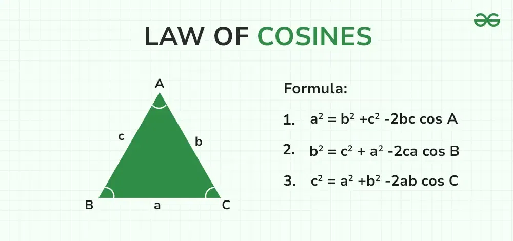
Which can be rewritten to compute angles as:
\(\Large \cos A = (\frac{b^2 + c^2 – a^2}{2bc})\)
\(\Large \cos B = (\frac{a^2 + c^2 – b^2}{2ac})\)
In our case:
\(a = L\)
\(b = tibia\)
\(c = femur\)
angle \(A = \Phi\)
angle \(B = \theta1\)
Therefore:
\(\Large \theta1 = \arccos(\frac{L^2 + femur^2 - tibia^2}{2 * L * femur})\)
or in python theta1 = math.acos((L**2 + femur**2 - tibia**2) / (2 * L * femur))
Similarly \(\Large \Phi = \arccos(\frac{tibia^2 + femur^2 - L^2}{2 * tibia * femur})\)
or in python phi = math.acos((tibia**2 + femur**2 - L**2) / (2 * tibia * femur))
What is left is to compute \(\beta\) and \(\gamma\) using the following formulas:
\(\beta = \theta1 + \theta2 - 90\) (offset by 90 degrees to align with leg coordinate frame, see diagram below of a straight leg)
\(\gamma = \Phi - 180\)
And that is all, lets put it all together:
def inverse_kinematics_xz(coxa, femur, tibia, foot_target, verbose=False):
    """
    XZ axis Inverse kinematics solver for 3DOF leg.

    Math as described above
    """
    D = -foot_target.y
    T = foot_target.x - coxa
    L = math.hypot(D, T)

    theta1 = math.degrees(math.acos((L**2 + femur**2 - tibia**2) / (2 * L * femur)))
    theta2 = math.degrees(math.atan2(T, D))
    phi = math.degrees(math.acos((tibia**2 + femur**2 - L**2) / (2 * tibia * femur)))

    beta = (theta1 + theta2) - 90
    gamma = phi - 180
    if verbose:
        print(f'{theta1=}\n{theta2=}\n{phi=}\n\n{beta=}\n{gamma=}')
    return beta, gamma


def solve_and_plot_at_target_xz(
    foot_target: Point, plot_title='Inverse Kinematics solved', verbose=False
):
    alpha = 0
    beta, gamma = inverse_kinematics_xz(
        coxa_len, femur_len, tibia_len, foot_target, verbose=verbose
    )

    model = forward_kinematics(
        coxa_len,
        femur_len,
        tibia_len,
        alpha,
        beta,
        gamma,
        # Inverse kinematic is defined in terms of leg coordinate frame, so body length and start_z are 0
        start_height=0,
        body_length=0,
    )

    fig, ax, _ = plot_leg_with_points(
        model,
        plot_title,
        joint_labels='points',
        x_label="X'",
        y_label='Z',
    )

    ax.scatter(foot_target.x, foot_target.y, color='k', label='Foot target')
    ax.legend().remove()
    return beta, gamma


alpha_ik, X_tick = coxa_ik(foot_target_3d.xy)

beta_ik, gamma_ik = solve_and_plot_at_target_xz(
    Point(X_tick, foot_target_3d.z), 'Foot_target_3D in XZ plane', verbose=True
)
display_and_close(plt.gcf())
theta1=59.92815342525586
theta2=67.99854209156905
phi=81.89132152492535

beta=37.92669551682491
gamma=-98.10867847507465

And that is all. We have solved inverse kinematics for a 3DOF leg.
print(f'alpha = {alpha_ik:.2f}')
print(f'beta = {beta_ik:.2f}')
print(f'gamma = {gamma_ik:.2f}')
alpha = 49.09
beta = 37.93
gamma = -98.11
To understand where the offset values for beta and gamma in the computation above are coming from, let’s plot straight leg and see what theta and phi are.
_ = solve_and_plot_at_target_xz(
    Point(coxa_len + femur_len + tibia_len, 0), 'Straight leg out', verbose=True
)
display_and_close(plt.gcf())
theta1=0.0
theta2=90.0
phi=180.0

beta=0.0
gamma=0.0

Now once we have the solution, let’s play with it a little bit and solve for various target points. If math is working correctly, foot (magenta dot) should always overlap with the target (black dot).
_ = solve_and_plot_at_target_xz(Point(20.61, 6.14), verbose=True)
display_and_close(plt.gcf())
theta1=56.45772587043364
theta2=111.47158023539903
phi=87.0052800205357

beta=77.92930610583267
gamma=-92.9947199794643

_ = solve_and_plot_at_target_xz(Point(15, 0), verbose=True)
display_and_close(plt.gcf())
theta1=88.85400800161142
theta2=90.0
phi=45.5729959991943

beta=88.85400800161142
gamma=-134.4270040008057

Putting it all together#
def inverse_kinematics(coxa, femur, tibia, foot_target: Point3D):
    alpha, X_tick = coxa_ik(foot_target.xy)
    beta, gamma = inverse_kinematics_xz(coxa, femur, tibia, Point(X_tick, foot_target.z))
    return alpha, beta, gamma
The classic IK test - drawing a circle#
The classic IK test is to draw a circle with the foot in each coordinate plane. Since we are using projects, let’s limit it to the XZ plane.
# Generate data and solve IK

steps = 32
x = 15.0
y = 0.0
z = -1.0
scalar = 2

sequence_xz_little_circle = [
    # x, y, z
    Point3D(x + math.sin(i) * scalar, y, z - math.cos(i) * scalar, f'xz-circle step {i}')
    for i in np.linspace(0, np.pi * 2, steps)
]
total_targets = len(sequence_xz_little_circle)

solved_foot = []
solved_model = []
for target in sequence_xz_little_circle:
    alpha, beta, gamma = inverse_kinematics(coxa_len, femur_len, tibia_len, target)
    model = forward_kinematics(
        coxa_len,
        femur_len,
        tibia_len,
        alpha,
        beta,
        gamma,
        # Inverse kinematic is defined in terms of leg coordinate frame, so body length and start_z are 0
        start_height=0,
        body_length=0,
    )
    foot = model[-1].end
    solved_foot.append(foot)
    solved_model.append(model)
# Plot IK solutions and targets into an animation


model = solved_model[0]

fig, ax, plot_data = plot_leg_with_points(
    model,
    'IK Circle',
    link_labels='none',
    joint_labels='points',
)


def animate(frame):
    even = not frame % 2
    if even:
        frame = frame // 2
        target = sequence_xz_little_circle[frame]
        ax.scatter(target.x, target.z, color='k', zorder=-100)
    else:
        frame = frame // 2
        model = solved_model[frame]
        plot_leg_update_lines(model, plot_data)
        foot = solved_foot[frame]
        ax.scatter(foot.x, foot.y, color='m', alpha=0.5, zorder=100)


_ = animate_plot(
    fig,
    animate,
    _interactive=False,
    _frames=total_targets * 2,
    _interval=50,
)
---------------------------------------------------------------------------
RuntimeError                              Traceback (most recent call last)
File ~/checkouts/readthedocs.org/user_builds/drqp/checkouts/latest/.venv/lib/python3.12/site-packages/IPython/core/formatters.py:406, in BaseFormatter.__call__(self, obj)
    404     method = get_real_method(obj, self.print_method)
    405     if method is not None:
--> 406         return method()
    407     return None
    408 else:

File ~/checkouts/readthedocs.org/user_builds/drqp/checkouts/latest/.venv/lib/python3.12/site-packages/matplotlib/animation.py:1385, in Animation._repr_html_(self)
   1383 fmt = mpl.rcParams['animation.html']
   1384 if fmt == 'html5':
-> 1385     return self.to_html5_video()
   1386 elif fmt == 'jshtml':
   1387     return self.to_jshtml()

File ~/checkouts/readthedocs.org/user_builds/drqp/checkouts/latest/.venv/lib/python3.12/site-packages/matplotlib/animation.py:1302, in Animation.to_html5_video(self, embed_limit)
   1299 path = Path(tmpdir, "temp.m4v")
   1300 # We create a writer manually so that we can get the
   1301 # appropriate size for the tag
-> 1302 Writer = writers[mpl.rcParams['animation.writer']]
   1303 writer = Writer(codec='h264',
   1304                 bitrate=mpl.rcParams['animation.bitrate'],
   1305                 fps=1000. / self._interval)
   1306 self.save(str(path), writer=writer)

File ~/checkouts/readthedocs.org/user_builds/drqp/checkouts/latest/.venv/lib/python3.12/site-packages/matplotlib/animation.py:121, in MovieWriterRegistry.__getitem__(self, name)
    119 if self.is_available(name):
    120     return self._registered[name]
--> 121 raise RuntimeError(f"Requested MovieWriter ({name}) not available")

RuntimeError: Requested MovieWriter (ffmpeg) not available
<matplotlib.animation.FuncAnimation at 0x73bc3b191a30>
Woohoo! The entire IK chain works as expected and we can put the foot on a target!
There is still one oopsy to cover, a case when the target is unreachable.
try:
    inverse_kinematics(1, 1, 1, Point3D(10, 1, 1))
except ValueError as e:
    print(e)
math domain error
The math domain error happens inside the acos function when input is outside of range [-1, 1] which happens exactly when there is no solution. One of the possible fixes is to cap the input to the valid range.
def safe_acos(num):
    if num < -1:
        return False, math.pi  # math.acos(-1)
    elif num > 1:
        return False, 0.0  # math.acos(1)
    else:
        return True, math.acos(num)


def sefe_inverse_kinematics_xz(coxa, femur, tibia, foot_target, verbose=False):
    """
    XZ axis Inverse kinematics solver for 3DOF leg.

    Math as described above
    """
    D = -foot_target.y
    T = foot_target.x - coxa
    L = math.hypot(D, T)

    solvable_theta1, theta1_rad = safe_acos((L**2 + femur**2 - tibia**2) / (2 * L * femur))
    theta1 = math.degrees(theta1_rad)

    theta2 = math.degrees(math.atan2(T, D))
    solvable_phi, phi_rad = safe_acos((tibia**2 + femur**2 - L**2) / (2 * tibia * femur))
    phi = math.degrees(phi_rad)

    beta = (theta1 + theta2) - 90
    gamma = phi - 180
    if verbose:
        print(
            f'{theta1=} - solvable={solvable_theta1}\n{theta2=}\n{phi=} - solvable={solvable_phi}\n\n{beta=}\n{gamma=}'
        )
    return solvable_theta1 and solvable_phi, beta, gamma


def safe_inverse_kinematics(coxa, femur, tibia, foot_target: Point3D, verbose=False):
    alpha, X_tick = coxa_ik(foot_target.xy)
    solvable, beta, gamma = sefe_inverse_kinematics_xz(
        coxa, femur, tibia, Point(X_tick, foot_target.z), verbose=verbose
    )
    return solvable, alpha, beta, gamma


try:
    solvable, alpha, beta, gamma = safe_inverse_kinematics(
        1, 1, 1, Point3D(10, 1, 1), verbose=True
    )
except ValueError as e:
    print(e)
theta1=0.0 - solvable=False
theta2=96.30553193947236
phi=180.0 - solvable=False

beta=6.30553193947236
gamma=0.0
With the safe capped version of acos function not only not throwing, but also provides a potential capped solution with properly reporting that actual solution is not possible.
Let’s plot it to have better intuition about what’s going on.
def safe_solve_and_plot_at_target(
    coxa,
    femur,
    tibia,
    foot_target: Point,
    plot_title='Inverse Kinematics',
    verbose=False,
):
    solvable, alpha, beta, gamma = safe_inverse_kinematics(
        coxa, femur, tibia, foot_target, verbose=verbose
    )

    model = forward_kinematics(
        coxa,
        femur,
        tibia,
        alpha,
        beta,
        gamma,
        # Inverse kinematic is defined in terms of leg coordinate frame, so body length and start_z are 0
        start_height=0,
        body_length=0,
    )

    _, ax, _ = plot_leg_with_points(
        model,
        plot_title + (' (target reached)' if solvable else ' (target unreachable)'),
        joint_labels='points',
        link_labels='none',
        x_label='X',
        y_label='Z',
    )
    xmin, xmax = ax.get_xlim()
    ax.set_xlim(min(xmin, foot_target.x - 1), max(xmax, foot_target.x + 1))
    ymin, ymax = ax.get_ylim()
    ax.set_ylim(min(ymin, foot_target.z - 1), max(ymax, foot_target.z + 1))

    ax.scatter(foot_target.x, foot_target.z, color='k', label='Foot target')

    tibia_line = model[-1]
    ax.plot(
        *zip(
            tibia_line.end,
            tibia_line.extended(np.linalg.norm((foot_target.xy - tibia_line.end).numpy())).end,
        ),
        'm:',
    )
    ax.legend().remove()


safe_solve_and_plot_at_target(1, 1, 1, Point3D(5, 0, -2), verbose=False)
display_and_close(plt.gcf())

The chart above is a nice demonstration of how the safe algorithm works. Even though leg is clearly not reaching the target (foot is the magenta dot), it is pointing exactly at the target as shown by the dotted line.